Artifact estimation network for MR images: effectiveness of batch normalization and dropout layers

Abstract

Background

Magnetic resonance imaging (MRI) is an essential tool for medical diagnosis. However, artifacts may degrade images obtained through MRI, especially owing to patient movement. Existing methods that mitigate the artifact problem are subject to limitations including extended scan times. Deep learning architectures, such as U-Net, may be able to address these limitations. Optimizing deep learning networks with batch normalization (BN) and dropout layers enhances their convergence and accuracy. However, the influence of this strategy on U-Net has not been explored for artifact removal.

Methods

This study developed a U-Net-based regression network for the removal of motion artifacts and investigated the impact of combining BN and dropout layers as a strategy for this purpose. A Transformer-based network from a previous study was also adopted for comparison. In total, 1200 images (with and without motion artifacts) were used to train and test three variations of U-Net.

Results

The evaluation results demonstrated a significant improvement in network accuracy when BN and dropout layers were implemented. The peak signal-to-noise ratio of the reconstructed images was approximately doubled and the structural similarity index was improved by approximately 10% compared with those of the artifact images.

Conclusions

Although this study was limited to phantom images, the same strategy may be applied to more complex tasks, such as those directed at improving the quality of MR and CT images. We conclude that the accuracy of motion artifact removal can be improved by integrating BN and dropout layers into a U-Net-based network, with due consideration of the correct location and dropout rate.

Background

Magnetic resonance imaging (MRI) is an effective and powerful method for the medical diagnosis of various conditions, such as tumors and blood flow abnormalities [1, 2]. Careful attention must be paid to image artifacts to achieve high diagnostic accuracy in MRI [3]. Image degradation owing to motion artifacts, such as those caused by respiratory and body motion, as well as pulsation, poses serious concerns such as poor diagnosis and prolonged examination times. Several mitigation measures have been proposed to address this issue.

First, respiratory gating was developed primarily to address image quality degradation caused by respiratory motion in upper abdominal imaging. The technique reduces the patient discomfort associated with breath-holding and substantially reduces the prevalence of motion artifacts [4]. Second, the periodically rotated overlapping parallel lines with enhanced reconstruction (PROPELLER) technique collects data from concentric rectangular strips rotated around the center of k-space. This method reduces the prevalence of motion artifacts by averaging the effects of low spatial frequency [5]. The limitations of these methods include the potential extension of scan times and an increased specific absorption rate associated with clinical imaging conditions, as well as the inability to apply the techniques retrospectively to images that have already been acquired. In recent years, deep learning has gained attention as a means of mitigating MRI artifacts and overcoming the aforementioned limitations. Fully convolutional networks, convolutional neural networks, and U-Net [6] are efficient deep learning networks that are used extensively for medical image segmentation and generation. Previous studies modified the U-Net layers to address artifacts [7,8,9].

Optimizing a deep learning network requires numerous trial-and-error attempts; however, the addition of batch normalization (BN) [10] and dropout layers [11] has been reported to facilitate convergence. These additions prevent model overfitting, enhance generalization, improve the segmentation capabilities, and increase robustness [12]. Zhao et al. improved the U-Net architecture by adding BN and dropout layers and optimizing the hyperparameters for accurate liver cell carcinoma segmentation [13]. However, the effects of incorporating BN and dropout layers into U-Net-based networks remain unexplored in terms of artifact removal. The potential of such an approach in facilitating the convergence of artifact-removal regression networks must be investigated.

In this study, we prototyped a regression network using U-Net as the backbone for motion artifact removal from images. In addition, we investigated the impacts of combining BN and dropout layers on the convergence and accuracy.

Methods

Overview

We acquired 1200 images through phantom scans, 600 each with motion artifacts (artifact images) and without motion artifacts (reference images). We computed the differences between the artifact images and reference images, thereby creating images that contained only the artifact components (difference images). We adjusted the presence and positioning of the BN and dropout layers and developed three networks for artifact component estimation. These networks were trained using pairs of reference and difference images. The output was visualized as estimated artifact components (estimated images). The results were compared with those of Transformer-based networks, which have exhibited superior results in previous studies. We calculated the peak signal-to-noise ratio (PSNR) and structural similarity index (SSIM) for all three variations and performed a statistical analysis.

Equipment and dataset

We used a MAGNETOM Prisma 3.0T MRI scanner (Siemens Healthcare) to image a multi-Carrageenan-Agarose-Gadolinium-NaCl (multi-CAGN) phantom (Kyoto Kagaku). MATLAB R2021b (MathWorks) was used for all analyses. The GPU used was a GEFORCE GTX 1070 (NVIDIA).

We captured 1200 T2-weighted 2D images, including artifact and reference images, by maintaining the same imaging conditions. Images with motion artifacts were obtained by randomly shaking the phantom during imaging. As the shape and relative positions of the components inside the phantom do not change with movement, the addition was a rigid motion artifact. We performed position corrections for both the artifact and reference images to account for structural misalignments other than artifacts. Sped-up robust features (features extracted solely from luminance gradients) were extracted and adjusted using the M-estimator Sample Consensus algorithm [14], which estimates the points of correspondence between images and transforms the angles and magnitudes corresponding to the point pairs. By subtracting the reference images from the artifact images, we created difference images containing only the artifact components. Of the 600 each of artifact and reference images, 580 were used for training, 10 for validation, and 10 for testing. These were converted into bitmap images to reduce the computational cost. An example of this procedure is shown in Figure 1. The imaging parameters were as follows: repetition time (TR): 4500 ms; echo time (TE): 75 ms; number of excitations (NEX): 2; bandwidth (BW): 300 Hz/pixel; flip angle (FA):150; echo train length (ETL): 16; slice thickness: 3 mm; field of view (FOV): 220 mm; phase resolution: 224/320.

Fig. 1

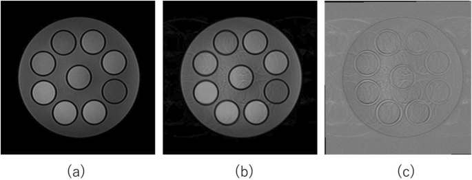
Example of dataset images (a) Reference image. (b) Artifact image. (c) Difference image. This figure shows an example image used in the training dataset. A difference image was created by subtracting the reference image from the artifact image after position correction

Network

We developed three variants of U-Net for artifact removal. The network created for this project incorporated three crucial factors (U-Net, BN, and dropout), as outlined below.

U-Net

U-Net was proposed in 2015 for medical image segmentation. It comprises an encoder-decoder architecture. During upsampling, the feature maps of the encoder are sent to the corresponding decoder layer, and the feature maps of the encoder and decoder are combined to complement the spatial information. The loss at the boundaries is increased so that the boundaries can be clearly distinguished, which requires image preprocessing to suit the intended purpose. In recent years, U-Net has also been used for image generation [15, 16]. A diagram of the proposed network is shown in Figure 2.

Fig. 2

Structure of the proposed networks. A schematic diagram of the proposed networks is shown. In Network 1, only the final layer was changed. In Network 2 and Network 3, a BN layer and a dropout layer were added, respectively

BN

In deep learning, bias within the activation function (output data after passing through the activation functions) can cause the vanishing gradient problem, leading to learning stagnation and a decrease in the representational capacity. This phenomenon may be addressed using BN. This technique adjusts the initial values of the weights and spreads the activation to fit a Gaussian distribution with a mean of 0 and a variance of 1.

Dropout

Dropout is a technique that is used to prevent overfitting by randomly deactivating nodes. The nodes that become inactive vary with each mini-batch. In deep learning, a mini-batch divides large datasets into smaller chunks, allowing for efficient utilization of memory and computational resources. By shuffling the training data and processing these in mini-batches, the approach significantly contributes to the rapid training of deep learning models, enhancing their efficiency in handling large datasets. The use of different combinations of active nodes during training improves the accuracy.

Developed networks

Considering the aforementioned specifications, we explored the efficiency of the networks in artifact removal. We selected U-Net as the base network for medical image processing. Tamada et al. investigated the motion artifact removal performance of deep learning networks [17]. They reported a method that subtracts artifact images from the images containing artifacts to reconstruct images. We followed a similar approach in this study. Specifically, during training, we paired artifact images with their corresponding difference images. This allowed for the creation of networks that can estimate only the artifact components when presented with artifact images as input. To improve U-Net, we incorporated dropout and BN layers and compared the performance across three different networks. We also adopted an improved Transformer network [2] used in a previous study [1], aimed at reducing motion artifacts, and compared it with these three networks.

Previous transformer network

A previous study by Lee et al. [18] examined motion artifact removal in head imaging by using a spatial transfer network [19] and a Transformer [20]. Johnson et al. [21] and Ulyanov et al. [22] proposed methods to improve the real-time performance of the Transformer. Lee et al. [18] obtained promising results by utilizing these improved Transformer networks in the motion artifact correction part of their experiments and compared their methods. Inspired by this previous study, we directly estimated the motion-free image by using images with motion artifacts as input. We herein refer to this network as the Transformer network.

Network 1

It was necessary to apply regression to the U-Net to generate images. Therefore, the softmax function, which is unnecessary for regression, was excluded, and a regression function was employed in the final layer. This modification was similarly applied to Network 2 and Network 3. No changes were applied to the other layers (Table 1).

Table 1 Layer structure of network 1

Network 2

Zhao et al. improved the robustness of U-Net by adding BN and dropout layers based on the U-Net architecture, thereby enhancing the model structure [13]. In general, the encoder repeatedly combines convolutional and pooling layers to reduce the resolution of the input image gradually while extracting highly abstract features. In Network 2, we applied BN and dropout (dropout rate: 0.1 or 0.2) after max pooling. In the decoder, a deconvolutional (upsampling) layer was applied to double the resolution to restore the compressed feature map to its original resolution. We placed a BN layer and dropout (dropout rate: 0.1 or 0.2) after the deconvolutional layer (Table 2). Consequently, the segmentation accuracy was improved for liver tumors [13]. This approach has the potential to effectively improve the image generation accuracy. The layer structure and dropout rate within the units applied to the tasks in this study were adapted from those by Zhang et al. [13].

Table 2 Layer structure of Network 2

Network 3

BN layers are typically used before and after the activation functions in a model. In addition, when combining BN and dropout layers, the dropout layers must be placed after the BN layers to avoid a decrease in accuracy [23]. The final layer of the decoder unit in U-Net is the activation function (the ReLU layer). Therefore, we added BN layers followed by dropout layers (dropout rate: 0.5) after the final ReLU function in the decoder and investigated their effectiveness (Table 3). The other layer structures were the same as those of Network 1.

Table 3 Layer structure of Network 3

Learning parameters

Transformer network parameters

Training was performed under the following conditions: the Adam optimizer was used, the initial learning rate was 0.001, the gradient decay coefficient was 0.01, the squared gradient decay coefficient was 0.999, the mini-batch size was 16, and the number of epochs was 50.

Three proposed networks parameters

Training was conducted under the following conditions: the Adam loss function was used, the initial learning rate was 0.001, the mini-batch size was 12, and the maximum number of epochs was 200. Adam is an optimization algorithm in deep learning that automatically adjusts the learning rates for efficient convergence. This method uses the exponential moving averages of past gradients and squared gradients to adjust the learning rates for individual parameters adaptively, ensuring fast convergence and reducing the likelihood of becoming stuck in local optima. Algorithms similar to Adam, such as RMSprop and Adagrad, also adjust the learning rates while providing suitable options for different problems and models. Moreover, we implemented early stopping: the training ended automatically when the validation root mean square error that was calculated every five epochs exceeded the previous value five consecutive times. The training was repeated five times for each network and the performance of each network was evaluated.

Evaluation

A total of 10 images were used for testing. We measured the SSIM and PSNR with respect to the reference images before and after artifact correction. SSIM is a metric used to measure the similarity between two images. It evaluates the perceived quality of images by comparing their luminance, contrast, and structure. A perfect match of the images will yield a score of 1.0. The PSNR is a metric that quantifies the quality of a reconstructed image compared to its original. It is expressed in decibels (dB) and is based on the logarithmic ratio of the maximum possible pixel value to the mean squared error (MSE) between the images. Higher PSNR values indicate better image quality. The SSIM and PSNR are expressed in Eqs. (1) and (2).

Representing the pixel values of image X as x, the pixel values of image Y as y, the mean pixel value of image X as ${\mu _x}$, the mean pixel value of image Y as ${\mu _y}$, the standard deviation of the pixel values of image X as ${\sigma _x}$, the standard deviation of the pixel values of image Y as ${\sigma _y}$, and the covariance of the pixel values between images X and Y as ${\sigma _{xy}}$, and employing ${C_1}$ and ${C_2}$ as constants to stabilize the output values, we obtain

$${\text{SSIM}}\,(x,y) = \frac{{\left( {2{\mu _x}{\mu _y} + {C_1}} \right)\left( {2{\sigma _{xy}} + {C_2}} \right)}}{{\left( {\mu _x^2 + \mu _y^2 + {C_1}} \right)\left( {\sigma _x^2 + \sigma _y^2 + {C_2}} \right)}}.$$

(1)

Representing the maximum pixel value as R and the MSE as MSE, we obtain

$${\rm{PSNR}} = {\rm{ }}10\,{\rm{lo}}{{\rm{g}}_{10}}{{{R^2}} \over {MSE}}{\rm{ }}$$

(2)

We calculated the average SSIM and PSNR values over five training runs for each network. To examine the significance of the values generated by the three networks, the Kruskal–Wallis test [24] (p < 0.05) was used, followed by the Steel Dwass post-hoc test.

Results

The average SSIM and PSNR values (over the five runs described in the previous section) for the 10 test images are listed in Tables 4 and 5, respectively. In the proposed method, the PSNR of the reconstructed images was approximately doubled and the SSIM was improved by approximately 10% compared with those of the artifact images. Box-and-whisker plots depicting the results of the significance tests are shown in Figs. 3 and 4 for the SSIM and PSNR, respectively. Both the SSIM and PSNR values differed significantly between Networks 1 and 2 as well as between Networks 1 and 3 (p < 0.01). No significant differences were observed between Networks 2 and Network 3. Significant differences were observed between the Transformer network and networks 1, 2, and 3. The estimated resulting images are shown in Fig. 5. Subfigures (d), (e), (f), and (g) show the estimated and corrected images for each network. In (d), the corrected image is estimated and the artifact components are calculated by subtracting the estimated corrected image from the motion image. In (e), (f), and (g), the artifact components are estimated and the corrected image is calculated by subtracting the estimated artifact components from the motion image. A visual inspection indicates that, compared with Fig. 1(b) and (c), the artifact estimation was successful for the networks other than the Transformer network and Network 1.

Table 4 PSNR values of test images

Table 5 SSIM values of test images

Fig. 3

Statistical analysis results of PSNR values. There was a significant difference between Networks 1 and 2 and between Networks 1 and 3 (p < 0.01). No significant difference was observed between Networks 2 and 3

Fig. 4

Statistical analysis results of SSIM values. A significant difference existed between Networks 1 and 2 and between Networks 1 and 3 (p < 0.01). No significant difference was observed between Networks 2 and 3

Fig. 5

Example results of estimated images. (a) Reference image. (b) Artifact image. (c) Difference image. (d) Transformer network. (e) Network 1. (f) Network 2. (g) Network 3. Each figure shows a pair of the artifact component image and the corrected image. The numbers in the center show the PSNR/SSIM of the image

Discussion

Both BN and dropout are techniques for mitigating overfitting. They are simple yet powerful approaches that contribute to improved accuracy; however, several considerations need to be made.

First, a key aspect is determining where to apply BN. The objective of BN is to achieve the stable distribution of activation values throughout the training process [10]. Consequently, although there is no general consensus regarding the optimal stage for applying BN, a prevalent approach is to implement it immediately before or after the activation function.

Second, the point at which the dropout is applied to each layer needs to be considered. Dropout is typically applied to fully connected layers because all features extracted from the convolutional and pooling layers are connected in a fully connected layer; therefore, applying dropout to this layer suppresses the influence of specific nodes on the output. However, Park et al. [25] analyzed the effects of dropout on convolutional layers, with the following results. Although the dropout rate was lower than that of the fully connected layer, positive results were also obtained by applying dropout to the convolutional layer. In the case of convolutional layers, dropout could render certain features inactive, implying a potential loss of information within the images. Therefore, selecting an appropriate dropout rate is crucial. Park et al. applied dropout after the activation function (ReLU) of each convolutional layer.

Finally, Li et al. [23] discussed the phenomenon of performance degradation when using dropout and BN simultaneously. The key to understanding the discord between dropout and BN lies in the discovered disparity in the behavior of variances during the transition from the training to the testing states in the network. Essentially, there is a difference in behavior between the learning and inference stages. Applying dropout before BN leads to different input variances, resulting in decreased accuracy. Therefore, applying the dropout layer after BN is necessary to circumvent these issues.

Based on these considerations, we discuss the networks created in this study. In Network 2, BN and dropout (with p = 0.1 or 0.2) were integrated before the convolutional layers used in U-Net. Previous studies have shown that this approach improves the segmentation accuracy. In this study, the approach was applied to an image estimation network for artifact removal and its effectiveness was established. This method moderately facilitated the transfer of features and facilitated learning convergence during image generation by maintaining a sufficiently low dropout coefficient in the convolutional layers. In Network 3, both BN and dropout (with p = 0.5) were added at the end of each decoder in U-Net. The final layers of the decoders typically use the ReLU activation function, which makes them suitable for incorporating BN. This modification led to improved convergence compared with Network 1 and enabled more accurate artifact estimation. This simple modification of U-Net resulted in a significant accuracy improvement.

Statistically, there was a significant difference in both the PSNR and SSIM values between Networks 1 and 2, and between Networks 1 and 3. The difference in the SSIM and PSNR between Networks 2 and 3 was approximately 1%, which was not large. The average training times for Networks 2 and 3 were approximately 100 min and 65 min, respectively. Considering the training time and network complexity, Network 3 proved to be the most useful.

The Transformer network did not improve the SSIM and PSNR significantly compared with the proposed network. Several points regarding the results should be noted. In the previous study [18], the “replacement of the central segment of k-space” was performed following motion correction. In this manner, the central space is replaced with the ground truth, i.e., the original contrast of the ground truth is guaranteed. This step could not be performed because the bitmap image format was used for training. The original paper reported that the images after this step had better evaluation scores. As can be observed from Fig. 5(d), the estimated images suggest that the contrast of the specimen in the phantom is lost. It is possible that the score can be improved by using DICOM images and performing k-space replacement. However, even when training using bitmap images, the average time to complete training exceeded approximately 8 h. It is clear that the calculation data would be even larger if DICOM images were used. One weakness of the transformer is that it is computationally expensive, and this point should be considered. Another shortcoming is that effective training requires a large amount of data and computational resources, and there is a high risk of overfitting on small datasets. The 560 images used to train the Transformer may not have been sufficient. If these points are addressed, the image quality and evaluation scores could be improved.

Although various motion artifact reduction networks have been reported, U-Net-based methods remain highly effective, as shown in prior research [26, 27]. Velayudham et al. developed a Transformer-based U-Net image pre-generator. They claimed that, using the U-Net structure, it is possible to remove noise at a high level [27]. Sadari et al. reported MRI motion artifact reduction using a conditional diffusion probabilistic model (MAR-CDPM) as a method for motion artifact reduction. MAR-CDPM uses a diffusion process that progressively increases the image distortion and then reverses this distortion to restore the original structure. Although this method preserves tumor boundaries and soft tissue contrast with excellent accuracy, it shows no significant difference in the artifact removal and distortion levels compared with supervised U-Net [26]. Our research also demonstrates the further potential of U-Net-based artifact reduction networks by employing dropout and BN layers. Medical images can vary in characteristics depending on the imaging conditions and equipment used. Therefore, patterns learned by a program may be difficult to apply to other datasets. This study used single-contrast (T2-weighted) imaging, but additional training may be necessary to adapt to different contrasts. Furthermore, this investigation was limited to a simple phantom image study. When considering future studies involving clinical images such as those captured from the human body, which require more complex learning, the complexity of the task is expected to be mitigated by BN and dropout. In addition, medical images often involve handling large volumes of data compared with those in the current study, necessitating efficient processing by the program. In this high computational load domain, high-performance hardware is often required and optimizing the program becomes a critical issue, especially when real-time processing is necessary.

Determining the network architecture and setting the hyperparameters remain challenging problems. Methods such as the grid search and random search, which are used to achieve high accuracy, require considerable time and effort [28]. The proposed approach, which involves adding BN and dropout layers to a basic network, is efficient for achieving convergence in deep learning and improving the accuracy. The technology developed in this study can also be applied to medical images, potentially contributing to improved images in various medical fields. Effective artifact removal is expected to eliminate the need for retakes and lengthy image reconstruction, thereby reducing examination times and the burden on patients.

Conclusions

Motion artifacts negatively affect MRI image quality. Deep learning architectures such as U-Net are considered as promising methods to prevent such degradation. In particular, a regression network was developed to remove motion artifacts effectively by applying the U-Net architecture that is specialized for segmentation. Furthermore, it was demonstrated that a BN layer and dropout layers could be effectively integrated into the design of this regression network. Consequently, the network stability improved and overfitting was prevented. In actual experiments and evaluations, this combination was confirmed to improve the accuracy significantly.

The results of this study demonstrate the possibility of not only successfully removing motion artifacts but also improving the accuracy and convergence speed of image processing using deep learning networks. We hope that future research and clinical applications will demonstrate the contribution of this method to improving the quality of MRI images.

References

Alvarez-Linera J. 3T MRI: advances in brain imaging. Eur J Radiol. 2008;67(3):415–26.
Lin DC, Wu KY, Sun FJ, Huang CC, Wu TH, Shih SL, et al. A quantitative image analysis using MRI for diagnosis of biliary atresia. Clin Imaging. 2019;53:186–90.
Takhtani D, Dundamadappa S, Puri AS, Wakhloo A. Flow artifact in the anterior communicating artery resembling aneurysm on the time of flight MR angiogram. Acta Radiol. 2014;55(10):1253–57.
Ehman RL, McNamara MT, Pallack M, Hricak H, Higgins CB. Magnetic resonance imaging with respiratory gating: techniques and advantages. AJR Am J Roentgenol. 1984;143:1175–82.
Pipe JG. Motion correction with PROPELLER MRI: application to head motion and free-breathing cardiac imaging. Magn Reson Med. 1999;42(5):963–69.
Ronneberger O, Fischer P, Brox T. U-Net: convolutional networks for biomedical image segmentation. Medical Image Computing and Computer-Assisted Intervention (MICCAI). 2015;234–41.
Jaubert O, Steeden J, Montalt-Tordera J, Arridge S, Kowalik GT, Muthurangu V. Deep artifact suppression for spiral real-time phase contrast cardiac magnetic resonance imaging in congenital heart disease. Magn Reson Imaging. 2021;83:125–32.
Abdi M, Feng X, Sun C, Bilchick KC, Meyer CH, Epstein FH. Suppression of artifact-generating echoes in cine DENSE using deep learning. Magn Reson Med. 2021;86(4):2095–104.
Hu R, Yang R, Liu Y, Li X. Simulation and mitigation of the wrap-around artifact in the MRI image. Front Comput Neurosci. 2021;15:746549.
Ioffe S, Szegedy C. Batch normalization: accelerating deep network training by reducing internal covariate. 2015. arXiv:1502.03167.
Srivastava N, Hinton G, Krizhevsky A, Sutskever I, Salakhutdinov R. Dropout: a simple way to prevent neural networks from overfitting. J Mach Learn Res. 2014;15(56):1929–58.
Hiasa Y, Otake Y, Takao M, Ogawa T, Sugano N, Sato Y. Automated muscle segmentation from clinical CT using Bayesian U-net for personalization of a musculoskeletal model. IEEE Trans Med Imaging. 2019;39(4):1030–40.
Zhao H, Wang Y, He C, Yang J, Shi Y, Zhu X. Automatic segmentation of magnetic resonance images of severe patients with advanced liver cancer and the molecular mechanism of emodin-induced apoptosis of HepG2 cells under the deep learning. J Healthcare Eng. 2022;2022:3951112. https://doiorg.publicaciones.saludcastillayleon.es/10.1155/2022/3951113.
Wu S, Zeng W, Chen H. A sub-pixel image registration algorithm based on SURF and M-estimator sample consensus. Pattern Recognit Lett. 2020;140:261–66.
Mizusawa S, Sei Y, Orihara R, Ohsuga A. Computed tomography image reconstruction using stacked U-Net. Comput Med Imaging Graph. 2021;90:101920.
Aghabiglou A, Eksioglu EM. Projection-based cascaded U-Net model for MR image reconstruction. Comput Methods Programs Biomed. 2021;207:106151.
Tamada D, Kromrey ML, Ichikawa S, Onishi H, Motosugi U. Motion artifact reduction using a convolutional neural network for dynamic contrast enhanced MR imaging of the liver. Magn Reson Med Sci. 2018;19(1):64–76.
Lee J, Seo H, Lee W, Park HW. Unsupervised motion artifact correction of turbo spin-echo MRI using deep image prior. Magn Reson Med. 2024;92(1):28–42.
Jaderberg M, Simonyan K, Zisserman A, Kavukcuoglu K. Spatial transformer networks. Adv Neural Inf Process Syst. 2015;28:2017–25.
Gatys LA, Ecker AS, Bethge M. Image style transfer using convolutional neural networks. In: The IEEE Conference on Computer Vision and Pattern Recognition (CVPR). 2016.
Johnson J, Alahi A, Fei-Fei L. arXiv:1603.08155. 2016.
Ulyanov D, Lebedev V, Vedaldi A, Lempitsky V. Texture networks: feed-forward synthesis of textures and stylized images. Proceedings of the 33rd International Conference on Machine Learning (ICML). 2016;48:1349–57.
Li X, Chen S, Hu X, Yang J. Understanding the Disharmony between Dropout and Batch Normalization by Variance Shift. 2018. arXiv:1801.05134.
Kruskal WH, Wallis WA. Use of ranks in one-criterion variance analysis. J Am Stat Assoc. 1952;47:583–621.
Park S, Kwak N. Analysis on the dropout effect in convolutional neural networks. In: Computer Vision– ACCV 2016. 2016.
Safari M, Yang X, Fatemi A, Archambault L. MRI motion artifact reduction using a conditional diffusion probabilistic model (MAR-CDPM). Med Phys. 2024;51(4):2598–610.
Velayudham A, Kumar KM, Priya MSK. Enhancing clinical diagnostics: novel denoising methodology for brain MRI with adaptive masking and modified non-local block. Med Biol Eng Comput. 2024;62:3043–56.
Liashchynskyi P, Liashchynskyi P. Grid search, random search, genetic algorithm: a big comparison for NAS. 2019. arXiv:1912.06059.
Acknowledgements
The authors wish to thank the editors from Editage for comments on earlier versions of this paper. In addition, we gratefully acknowledge the work of past and present members of our laboratory.
Funding
No funds, grants, or other support were received.
Author information
Authors and Affiliations
Contributions
All authors contributed to the study conception and design. Material preparation, data collection, and analysis were performed by Tomoko Maruyama. The first draft of the manuscript was written by Tomoko Maruyama and all authors commented on previous versions of the manuscript. All authors read and approved the final manuscript.
Corresponding author
Ethics declarations
Ethics approval and consent to participate
This article does not contain any studies with human participants or animals performed by any of the authors.
Consent for publication
Not applicable.
Competing interests
The authors declare no competing interests.
Additional information
Publisher’s Note
Springer Nature remains neutral with regard to jurisdictional claims in published maps and institutional affiliations.
Electronic supplementary material
Below is the link to the electronic supplementary material.
Rights and permissions
Open Access This article is licensed under a Creative Commons Attribution-NonCommercial-NoDerivatives 4.0 International License, which permits any non-commercial use, sharing, distribution and reproduction in any medium or format, as long as you give appropriate credit to the original author(s) and the source, provide a link to the Creative Commons licence, and indicate if you modified the licensed material. You do not have permission under this licence to share adapted material derived from this article or parts of it. The images or other third party material in this article are included in the article’s Creative Commons licence, unless indicated otherwise in a credit line to the material. If material is not included in the article’s Creative Commons licence and your intended use is not permitted by statutory regulation or exceeds the permitted use, you will need to obtain permission directly from the copyright holder. To view a copy of this licence, visit http://creativecommons.org/licenses/by-nc-nd/4.0/.
About this article
Cite this article
Maruyama, T., Hayashi, N., Sato, Y. et al. Artifact estimation network for MR images: effectiveness of batch normalization and dropout layers. BMC Med Imaging 25, 144 (2025). https://doiorg.publicaciones.saludcastillayleon.es/10.1186/s12880-025-01663-8
Received:
Accepted:
Published:
DOI: https://doiorg.publicaciones.saludcastillayleon.es/10.1186/s12880-025-01663-8